Functional Sets, Part 1: Construction
Before we start for real, what’s a set?
Say we have the numbers 1 through 4.
In a list, that’s easy enough: [1, 2, 3, 4].
And, in a set, it’s still [1, 2, 3, 4].
The difference comes with duplicate elements: four ones in a list is [1, 1, 1, 1], but in a set that’s just [1].
Sets don’t respect order, either: [4, 3, 2, 1] and [1, 2, 3, 4] are the same set.
Instead of order, we talk about membership.
The set has four items: 1, 2, 3, and 4 (or, if you prefer: 4, 3, 2, and 1.)
You can use sets for tons of neat things! Relational databases use sets as the basis for operation, and TLA+ uses set logic to do formal verification of software. If you’d like to find out more about set theory later, Wikipedia has got your back.
What are our sets made of?
We’re going to implement our Sets with binary search trees. A binary search tree containing the numbers 1, 2, and 3 might look like this:
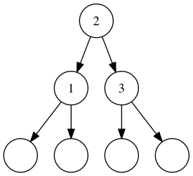
A binary search tree containing 1, 2, and 3. Empty circles represent empty trees.
An element in this particular data structure has a head (the top node) and two sub-elements, or sub-trees. The left tree contains items less than the head, and the right tree contains items greater than the head. If there are no items less than or greater than the head, the trees below it are empty.
In the example above 2 is the head, with 1 on the left and 3 on the right. We don’t have any values other than those three, so the other subtrees are all empty.
This all sounds kiiiiind of complicated. Why are we using this particular data structure? Well, think about this: if a node can contain one value, and things greater and less than that value, then we have disallowed duplicate items. We didn’t have to write complicated code to do this, we just had to choose a structure that made impossible states (duplicate values) unrepresentable!
The Data Model
Enough theory! How does this look in actual code?
type Set comparable
    = Tree comparable (Set comparable) (Set comparable)
    | Empty
This is a type union with two tags: Tree and Empty.
We’ll use Empty to represent an empty set, and Tree to represent a non-empty set (with potentially non-empty left and right subtrees.)
Our Set type takes a comparable as part of the type.
comparable refers to any type whose values we can compare, for example 1 < 2 or 'c' > 'a'.
In Elm, this means we can use Int, Float, Time, Char, String, and tuples or lists of those types.
This data structure can represent every tree imaginable. For example:
- An empty set:
Empty - A set with just 1 in it:
Tree 1 Empty Empty - Our example with 1, 2, and 3:
Tree 2 (Tree 1 Empty Empty) (Tree 3 Empty Empty)
But even with three values, creating these by hand gets a little hairy, so let’s make some basic constructor functions:
empty : Set comparable
empty =
    Empty

singleton : comparable -> Set comparable
singleton item =
    Tree item empty empty
That’s better. So now:
- An empty set:
empty - A set with just 1 in it:
singleton 1 - A set with 1, 2, and 3:
Tree 2 (singleton 1) (singleton 3)
These functions make constructing simple sets easier, but what about more complex things? Even 1 through 3 is still too complex for everyday use! We don’t want to track whether to place things on the left or the right for every single set, right? Lucky for us, that’s where insertion comes in:
Inserting
We’ll want a function that will insert a new value into our set… so, being extremely creative we call it insert.
Let’s dive into the code, and I’ll explain as we go:
insert : comparable -> Set comparable -> Set comparable
insert item set =
    case set of
        Empty ->
            singleton item

        Tree head left right ->
            if item < head then
                Tree head (insert item left) right
            else if item > head then
                Tree head left (insert item right)
            else
                set
First, we need to determine if the set is empty.
If we’ve got an empty list, we don’t need to worry about inserting on the left or the right; we can just create a new singleton!
Otherwise, we need to compare the head with the new item:
- If the item we’re inserting is less than the head, we insert into the left set.
- If it’s greater, we insert into the right set.
- If the two values are equal, we do nothing. The item is already present, so don’t make any changes!
Then, after we’ve figured out where we insert, we’ll do it again for the next level until we get to either a level that doesn’t have a value (empty) or a value we’ve already seen.
Recursive code like this can be tricky to understand, so let’s visualize what’s happening.
Let’s say we want to insert 0 into a singleton set containing 1.
We’ll call insert 0 (singleton 1):
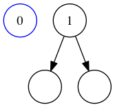
A singleton set containing 1, and a new value 0.
We compare to the singleton set in the pattern matching.
Now we’re comparing the item we’re inserting (0) to the head of the current tree (1):
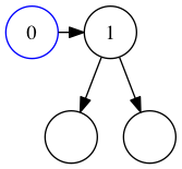
Comparing the inserted value to the head.
We find that 0 is less than 1, so insert the new item to the left.
This is the same as calling insert 0 Empty, since the left node is empty.
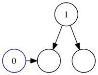
Comparing the inserted value to the left branch.
This time around, the set in question is Empty, so we’ll return a new singleton.
Our new set then bubbles up through the recursive calls.
It ends up replacing the left branch of the original set.
The original call returns with the modified set, and we’re finished.
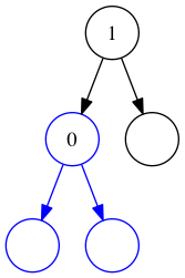
The final tree, with the new value inserted.
List to Set
Now, that takes care of inserting a single value, but what if you have a list?
All it takes is List.foldl!
fromList : List comparable -> Set comparable
fromList items =
    List.foldl insert empty items
To put this in English: starting from the beginning, insert the items one at a time into a new set.
This is the functional equivalent of a for loop with an accumulator.
Conversion function: complete!
So Far
To sum up: we’ve got:
- a recursively defined Set data structure
- constructors for both kinds of base values (empty sets and singleton sets)
- two ways to insert values into sets (
insertandfromList)
We’ve got a good foundation, but we have quite a way to go. Next time we’ll going to look at how to tell if a set contains a value. We’ll also cover how to measure how many values are in our set.